Legend Behavior in Data Visualization: Automatic Labeling and Updates

152

The legend function creates a legend with descriptive labels for each plotted data series. It uses the DisplayName property of the data series for labels. If DisplayName is empty, a default label in the format 'dataN' is used. The legend updates automatically when data series are added or removed. It is created in the current axes, as returned by gca. If the axes are empty, the legend remains empty. If no axes exist, legend generates Cartesian axes.

Syntax and Usage

• legend(label1, ..., labelN): Sets custom legend labels using character vectors or strings, e.g., legend('Jan', 'Feb', 'Mar').
• legend(labels): Uses a cell array, string array, or character matrix for labels, e.g., legend({'Jan', 'Feb', 'Mar'}).
• legend(subset,___): Displays only selected data series in the legend, where subset is a vector of graphics objects.
• legend(target,___): Creates a legend for a specified target (axes or standalone visualization) instead of the current axes.
• legend(___, 'Location', lcn): Sets the legend position, e.g., 'northeast' places it in the upper-right corner.
• legend(___, 'Orientation', ornt): Specifies legend layout as 'horizontal' (side-by-side) or 'vertical' (default).
• legend(___, Name, Value): Configures legend properties using name-value pairs.
• legend(bkgd): Controls background visibility, where 'boxoff' hides the legend background and outline, while 'boxon' (default) displays them.
• lgd = legend(___): Returns the Legend object, allowing further property modifications.
• legend(vsbl): Controls visibility using 'hide', 'show', or 'toggle'.
• legend('off'): Deletes the legend.

Add Legend to Current Axes

x = linspace(0,pi);
y1 = cos(x);
plot(x,y1)

hold on 
y2 = cos(2*x);
plot(x,y2)

legend('cos(x)','cos(2x)')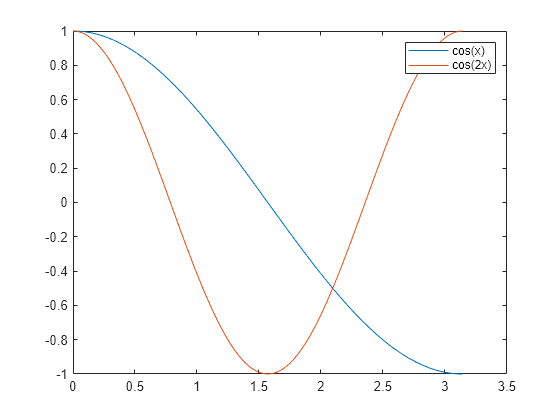

If you add or remove a data series from the axes, the legend updates automatically. To control the label of a new data series, set the DisplayName property as a name-value pair during creation. If no label is specified, the legend assigns a default label in the format 'dataN'.

Note: To prevent the legend from updating when data series are added or removed, set the AutoUpdate property of the legend to 'off'.

y3 = cos(3*x);
plot(x,y3,'DisplayName','cos(3x)')
hold off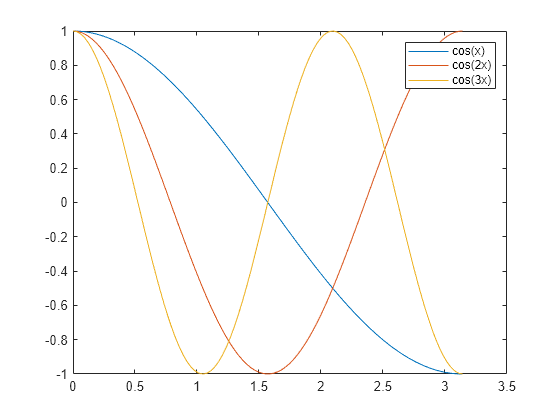

Delete the legend. Get 

legend('off')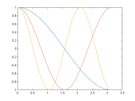

Add Legend to Specific Axes

You can arrange multiple plots using the tiledlayout and nexttile functions. First, use tiledlayout to create a 2-by-1 grid layout. Then, call nexttile to generate the axes objects ax1 and ax2. Plot random data in each axes. To add a legend to the upper plot, pass ax1 as the first argument to legend.

tiledlayout(2,1)
y1 = rand(3);
ax1 = nexttile; 
plot(y1)

y2 = rand(5);
ax2 = nexttile; 
plot(y2)

legend(ax1,{'Line 1','Line 2','Line 3'})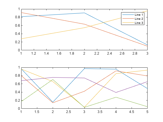

Specify Legend Labels During Plotting Commands

Plot two lines and set the DisplayName property to specify legend labels during the plotting commands. Finally, add a legend to display the labels.

x = linspace(0,pi);
y1 = cos(x);
plot(x,y1,'DisplayName','cos(x)')

hold on 
y2 = cos(2*x);
plot(x,y2,'DisplayName','cos(2x)')
hold off

legend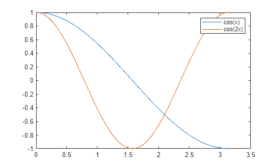

Exclude Line from Legend

To exclude a line from the legend, set its label as an empty character vector or string. For example, plot two sine waves and add a dashed zero line using the yline function. Then, create a legend while omitting the zero line by setting its label to ”.

x = 0:0.2:10;
plot(x,sin(x),x,sin(x+1));
hold on
yline(0,'--')
legend('sin(x)','sin(x+1)','')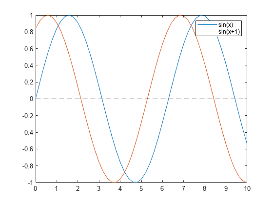

List Entries in Columns and Specify Legend Location

Plot four lines and add a legend in the northwest corner of the axes. Use the NumColumns property to specify the number of columns in the legend.

x = linspace(0,pi);
y1 = cos(x);
plot(x,y1)

hold on
y2 = cos(2*x);
plot(x,y2)

y3 = cos(3*x);
plot(x,y3)

y4 = cos(4*x);
plot(x,y4)
hold off

legend({'cos(x)','cos(2x)','cos(3x)','cos(4x)'},...
    'Location','northwest','NumColumns',2)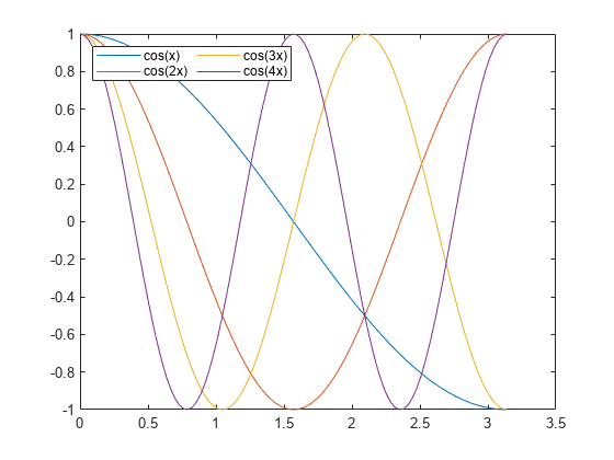

Reverse Order of Legend Items

Starting from R2023b, you can reverse the order of legend items by adjusting the Direction property of the legend. For example, plot four lines and add a legend.

plot([4 5 6 7; 0 1 2 3])
lgd = legend("First","Second","Third","Fourth");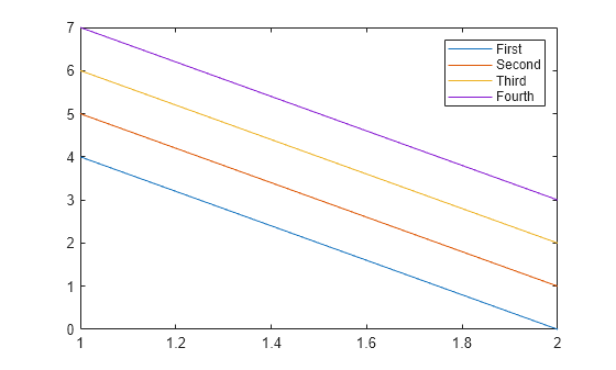

Reverse the order of the legend items. Get 

lgd.Direction = "reverse";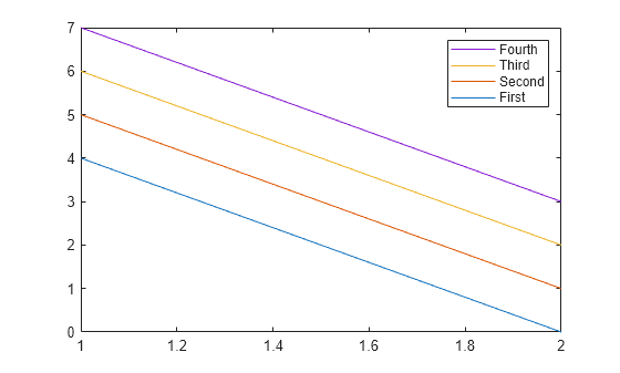

Display Shared Legend in Tiled Chart Layout

If you wish to share a legend across multiple plots, you can display the legend in a separate tile within the layout. It can either be placed within the grid of tiles or in an outer tile.

To create three plots in a tiled chart layout:

t = tiledlayout('flow','TileSpacing','compact');
nexttile
plot(rand(5))
nexttile
plot(rand(5))
nexttile
plot(rand(5))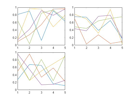

lgd = legend;
lgd.Layout.Tile = 4;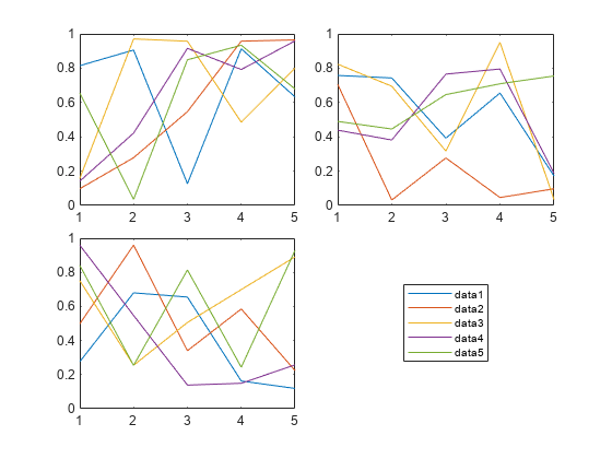

Next, add a fourth plot and move the legend to the east tile. Get 

nexttile
plot(rand(5))
lgd.Layout.Tile = 'east';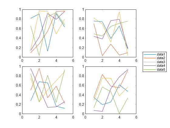

Included Subset of Graphics Objects in Legend

If you want to exclude some of the plotted graphics objects from the legend, you can specify only the ones you wish to include.

For example, plot three lines and store the created Line objects. Then, create a legend that includes just two of the lines. You can do this by passing a vector of the desired Line objects as the first input argument.

x = linspace(0,pi);
y1 = cos(x);
p1 = plot(x,y1);

hold on
y2 = cos(2*x);
p2 = plot(x,y2);

y3 = cos(3*x);
p3 = plot(x,y3);
hold off

legend([p1 p3],{'First','Third'})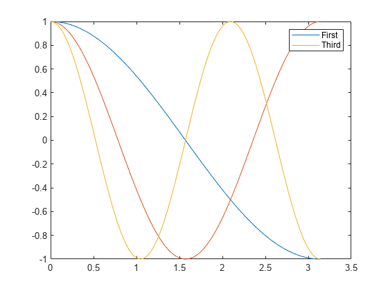

Create Legend with LaTeX Markup

Create a plot and add a legend with LaTeX formatting by calling the legend function and setting the Interpreter property to ‘latex’. Enclose the LaTeX markup within dollar signs ($).

x = 0:0.1:10;
y = sin(x);
dy = cos(x);
plot(x,y,x,dy);
legend('$sin(x)$','$\frac{d}{dx}sin(x)$','Interpreter','latex');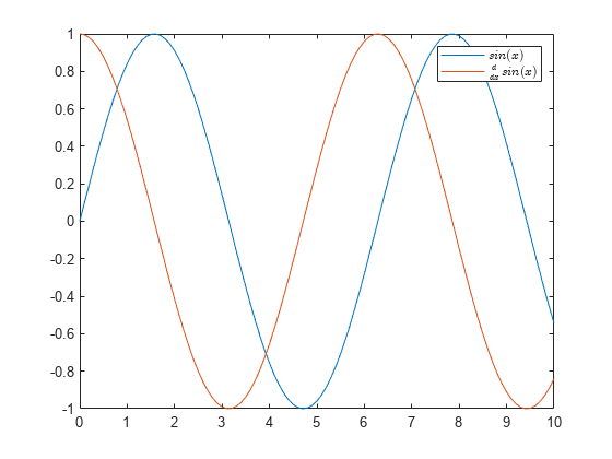

Add Title to Legend

x = linspace(0,pi);
y1 = cos(x);
plot(x,y1)

hold on
y2 = cos(2*x);
plot(x,y2)
hold off

lgd = legend('cos(x)','cos(2x)');
title(lgd,'My Legend Title')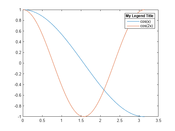

Remove Legend Background

x = linspace(0,pi);
y1 = cos(x);
plot(x,y1)

hold on
y2 = cos(2*x);
plot(x,y2)
hold off

legend({'cos(x)','cos(2x)'},'Location','southwest')
legend('boxoff')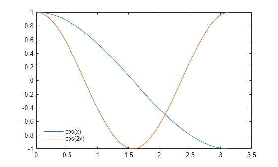

Specify Legend Font Size and Color

You can modify various aspects of a legend by adjusting its properties. These properties can be set either by providing name-value pairs when calling the legend function, or by modifying the properties of the Legend object after it has been created.

Example:

Plot four lines of random data, create a legend, and assign the Legend object to the variable lgd. Then, adjust the FontSize and TextColor properties using name-value arguments.

rdm = rand(4);
plot(rdm)

lgd = legend({'Line 1','Line 2','Line 3','Line 4'},...
    'FontSize',12,'TextColor','blue');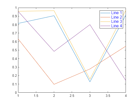

lgd.NumColumns = 2;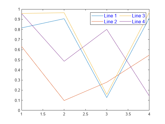

Specify Width of Legend Icons

Starting from R2024b, you can adjust the width of the legend icons by setting the IconColumnWidth property. For instance, plot a line along with two sets of scattered data.

% Create the data
x = 1:50;
sample1 = x + randn(1,50);
sample2 = (x-5) + randn(1,50); 
y = x - 10;

% Plot the data
plot(x,y)
hold on
scatter(x,sample1,"filled")
scatter(x,sample2,"filled")
hold off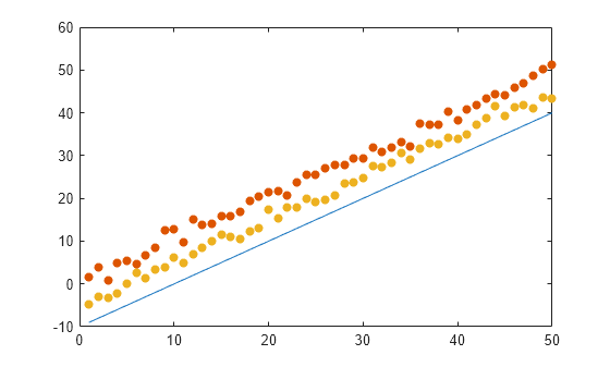

lgd = legend("Expected","Sample 1","Sample 2");
lgd.Location = "north";
lgd.Orientation = "horizontal";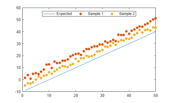

Reduce the width of the icon column by setting the IconColumnWidth property to 10. This will shorten the line icon and minimize the space around the markers.

lgd.IconColumnWidth = 10;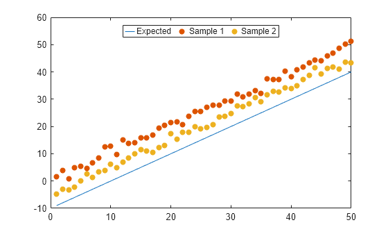

Input Arguments

Labels (as Separate Arguments)

Character Vectors | Strings
Labels are provided as a comma-separated list of character vectors or strings.

• To exclude an item from the legend, provide an empty string or character vector as its label.
• For special characters or Greek letters, use TeX or LaTeX markup. For a full list of options, refer to the Interpreter property.

Examples:

• legend('Sin Function','Cos Function')
• legend("Sin Function","Cos Function")
• legend("Sample A","","Sample C")
• legend('\gamma','\sigma')

Labels (as an Array)

Cell Array of Character Vectors | String Array | Categorical Array
Labels specified in a cell array, string array, or categorical array.

• To exclude an item from the legend, set the corresponding label as an empty string or character vector in the array.
• Special characters or Greek letters can be included using TeX or LaTeX markup. See the Interpreter property for options.

Examples:

• legend({'Sin Function','Cos Function'})
• legend(["Sin Function","Cos Function"])
• legend({'Sample A','','Sample C'})
• legend({'\gamma','\sigma'})
• legend(categorical({'Alabama','New York'}))

Subset — Data Series to Include in Legend

Vector of Graphics Objects
Specifies which data series should appear in the legend, provided as a vector of graphics objects.

Target — Target for Legend

Axes Object | PolarAxes Object | GeographicAxes Object | Standalone Visualization
Defines the target for the legend. This can be an Axes object, PolarAxes object, GeographicAxes object, or a standalone visualization (e.g., a GeographicBubbleChart object).
If not specified, the legend will apply to the object returned by gca.

Note: Standalone visualizations do not support modifications to legend appearance (e.g., location changes) or returning the Legend object.

lcn — Legend location

'north' | 'south' | 'east' | 'west' | 'northeast' | ...

Here’s the table you requested:

Value	Description
‘north’	Inside top of axes
‘south’	Inside bottom of axes
‘east’	Inside right of axes
‘west’	Inside left of axes
‘northeast’	Inside top-right of axes (default for 2-D axes)
‘northwest’	Inside top-left of axes
‘southeast’	Inside bottom-right of axes
‘southwest’	Inside bottom-left of axes
‘northoutside’	Above the axes
‘southoutside’	Below the axes
‘eastoutside’	To the right of the axes
‘westoutside’	To the left of the axes
‘northeastoutside’	Outside top-right corner of the axes (default for 3-D axes)
‘northwestoutside’	Outside top-left corner of the axes
‘southeastoutside’	Outside bottom-right corner of the axes
‘southwestoutside’	Outside bottom-left corner of the axes
‘best’	Inside axes where least conflict occurs with the plot data at the time the legend is created. May need reset if the plot data changes.
‘bestoutside’	Outside top-right corner of the axes (vertical orientation) or below the axes (horizontal orientation)
‘layout’	A tile in a tiled chart layout. Set the Layout property of the legend to move it to a different tile.
‘none’	Determined by Position property. Use the Position property for a custom location.

ornt — Orientation

‘vertical’ (default) | ‘horizontal’
Specifies the orientation of the legend items:

• ‘vertical’ — Displays the legend items stacked vertically.
• ‘horizontal’ — Lists the legend items side-by-side.

Example:
legend('Orientation','horizontal')

bkgd — Legend Box Display

‘boxon’ (default) | ‘boxoff’
Controls the display of the legend box:

• ‘boxon’ — Displays the legend background and outline.
• ‘boxoff’ — Hides the legend background and outline.

Example:
legend('boxoff')

vsbl — Legend Visibility

‘hide’ | ‘show’ | ‘toggle’
Specifies the visibility of the legend:

• ‘hide’ — Hides the legend.
• ‘show’ — Displays the legend, or creates one if it doesn’t exist.
• ‘toggle’ — Toggles the visibility of the legend.

Example:
legend('hide')

Name-Value Arguments

Optional pairs of arguments can be specified in the format Name1=Value1, ..., NameN=ValueN. The Name is the argument name, and Value is the corresponding value. The order of the name-value pairs does not matter, but they must appear after other arguments.

Example:
legend({'A','B'},'TextColor','blue','FontSize',12)
This creates a legend with blue text and 12-point font size.

TextColor — Text Color

[0 0 0] (default) | RGB triplet | hexadecimal color code | ‘r’ | ‘g’ | ‘b’ | …
Specifies the color of the text. The default color is black, represented by the RGB triplet [0 0 0].

You can define the text color using one of the following methods:

• RGB Triplet: A three-element row vector that represents the intensities of the red, green, and blue components of the color. The values must range from [0,1]. For example, [0.4 0.6 0.7].
• Hexadecimal Color Code: A string or character vector starting with a hash symbol (#), followed by three or six hexadecimal digits (0-9, A-F). Hexadecimal values are case-insensitive. For instance, "#FF8800", "#ff8800", "#F80", and "#f80" are equivalent.
• Color Name: You can also specify common colors using their names (e.g., 'r' for red, 'g' for green, 'b' for blue).

Color Name	Short Name	RGB Triplet	Hexadecimal Color Code	Appearance
"red"	"r"	[1 0 0]	"#FF0000"
"green"	"g"	[0 1 0]	"#00FF00"
"blue"	"b"	[0 0 1]	"#0000FF"
"cyan"	"c"	[0 1 1]	"#00FFFF"
"magenta"	"m"	[1 0 1]	"#FF00FF"
"yellow"	"y"	[1 1 0]	"#FFFF00"
"black"	"k"	[0 0 0]	"#000000"
"white"	"w"	[1 1 1]	"#FFFFFF"
"none"	Not applicable	Not applicable	Not applicable	No color

Here are the RGB triplets and hexadecimal color codes for the default colors MATLAB^® uses in many types of plots.

RGB Triplet	Hexadecimal Color Code	Appearance
[0 0.4470 0.7410]	"#0072BD"
[0.8500 0.3250 0.0980]	"#D95319"
[0.9290 0.6940 0.1250]	"#EDB120"
[0.4940 0.1840 0.5560]	"#7E2F8E"
[0.4660 0.6740 0.1880]	"#77AC30"
[0.3010 0.7450 0.9330]	"#4DBEEE"
[0.6350 0.0780 0.1840]	"#A2142F"

Example: [0 0 1]

Example: 'blue'

Example: '#0000FF'

FontSize — Font Size

Scalar value greater than zero
Specifies the font size in point units, where the value must be greater than zero. The default font size depends on the operating system and locale.

When you change the font size of the axes, MATLAB automatically adjusts the font size of the colorbar to 90% of the axes font size. However, if you manually set the colorbar font size, changes to the axes font size will not affect the colorbar.

NumColumns — Number of Columns

1 (default) | Positive integer
Defines the number of columns in the legend, specified as a positive integer. If there are fewer legend items than the specified number of columns, the actual number of columns may be less.

You can control whether the legend items are arranged by column or row using the Orientation property.

Example:
lgd.NumColumns = 3

Output Arguments

lgd — Legend Object

Returns the legend object, which can be used to view or modify legend properties after it has been created.

lgd — Legend object
Legend object

Legend object. Use lgd to view or modify properties of the legend after it is created.

plot(rand(3))
lgd = legend('line1','line2','line3');
lgd.FontSize = 12;
lgd.FontWeight = 'bold';