Greek Letters and Special Characters in Chart Text

36

You can enhance chart text by including Greek letters and special characters through TeX markup. This also allows you to add superscripts, subscripts, and customize text types and colors. MATLAB® natively supports a subset of TeX markup, but for more advanced symbols like integrals and summations, you can switch to LaTeX markup. In the following example, we demonstrate how to insert Greek letters, superscripts, and annotations into your chart text, while also highlighting other available TeX formatting options.

Include Greek Letters

To include Greek letters in a MATLAB plot, you can use TeX markup in the title. For example, to add the Greek letter π in the title of a simple line plot, use the \pi symbol in the title string.

Here’s how to do it:

x = linspace(0,2*pi);
y = sin(x);
plot(x,y)
title('x ranges from 0 to 2\pi')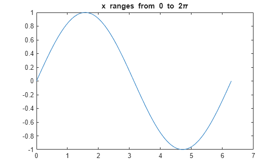

Include Superscripts and Annotations

To enhance your line plot, add a title and axis labels, and display superscripts using the ^ character. The ^ character applies to the character immediately following it, and you can include multiple characters in the superscript by enclosing them in curly braces {}.

Additionally, you can incorporate Greek letters such as α and μ in your text by using TeX markups like \alpha and \mu, respectively.

For example, to display a superscript and Greek letters in the title, you can write:

t = 1:900;
y = 0.25*exp(-0.005*t);

figure
plot(t,y)
title('Ae^{\alphat} for A = 0.25 and \alpha = -0.0005')
xlabel('Time')
ylabel('Amplitude')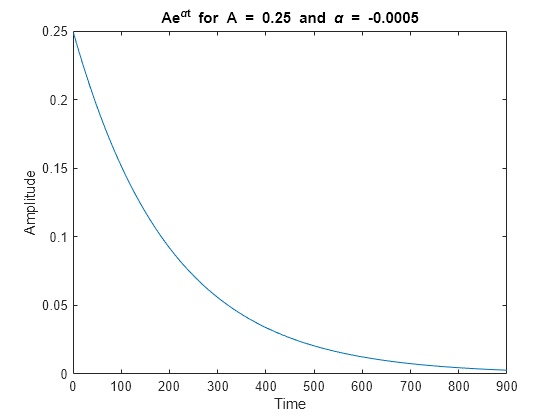

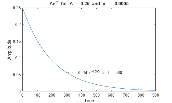
Add Text at the Data Point Where t = 300

To add text at a specific data point where t = 300, use TeX markup to include a bullet marker and an arrow pointing to the left. By default, the text will appear to the left of the data point.

Here’s how you can do it:

txt = '\bullet \leftarrow 0.25t e^{-0.005t} at t = 300';
text(t(300),y(300),txt)

TeX Markup Options

MATLAB supports a subset of TeX markup, allowing you to enhance your plot’s text by adding superscripts, subscripts, changing the text type and color, and including special characters. To make use of TeX markup, ensure that the Interpreter property of the text object is set to ‘tex’ (which is the default setting).

Modifiers will remain active until the end of the text, with the exception of superscripts and subscripts, which only apply to the next character or to characters enclosed in curly braces. When the interpreter is set to ‘tex’, the following modifiers are supported:

Modifier	Description	Example
^{ }	Superscript	'text^{superscript}'
_{ }	Subscript	'text_{subscript}'
\bf	Bold font	'\bf text'
\it	Italic font	'\it text'
\sl	Oblique font (usually the same as italic font)	'\sl text'
\rm	Normal font	'\rm text'
\fontname{specifier}	Font name — Replace specifier with the name of a font family. You can use this in combination with other modifiers.	'\fontname{Courier} text'
\fontsize{specifier}	Font size —Replace specifier with a numeric scalar value in point units.	'\fontsize{15} text'
\color{specifier}	Font color — Replace specifier with one of these colors: red, green, yellow, magenta, blue, black, white, gray, darkGreen, orange, or lightBlue.	'\color{magenta} text'
\color[rgb]{specifier}	Custom font color — Replace specifier with a three-element RGB triplet.	'\color[rgb]{0,0.5,0.5} text'

This table lists the supported special characters for the 'tex' interpreter.

Character Sequence	Symbol	Character Sequence	Symbol	Character Sequence	Symbol
\alpha	α	\upsilon	υ	\sim	~
\angle	∠	\phi	ϕ	\leq	≤
\ast	*	\chi	χ	\infty	∞
\beta	β	\psi	ψ	\clubsuit	♣
\gamma	γ	\omega	ω	\diamondsuit	♦
\delta	δ	\Gamma	Γ	\heartsuit	♥
\epsilon	ϵ	\Delta	Δ	\spadesuit	♠
\zeta	ζ	\Theta	Θ	\leftrightarrow	↔
\eta	η	\Lambda	Λ	\leftarrow	←
\theta	θ	\Xi	Ξ	\Leftarrow	⇐
\vartheta	ϑ	\Pi	Π	\uparrow	↑
\iota	ι	\Sigma	Σ	\rightarrow	→
\kappa	κ	\Upsilon	ϒ	\Rightarrow	⇒
\lambda	λ	\Phi	Φ	\downarrow	↓
\mu	µ	\Psi	Ψ	\circ	º
\nu	ν	\Omega	Ω	\pm	±
\xi	ξ	\forall	∀	\geq	≥
\pi	π	\exists	∃	\propto	∝
\rho	ρ	\ni	∍	\partial	∂
\sigma	σ	\cong	≅	\bullet	•
\varsigma	ς	\approx	≈	\div	÷
\tau	τ	\Re	ℜ	\neq	≠
\equiv	≡	\oplus	⊕	\aleph	ℵ
\Im	ℑ	\cup	∪	\wp	℘
\otimes	⊗	\subseteq	⊆	\oslash	∅
\cap	∩	\in	∈	\supseteq	⊇
\supset	⊃	\lceil	⌈	\subset	⊂
\int	∫	\cdot	·	\o	ο
\rfloor	⌋	\neg	¬	\nabla	∇
\lfloor	⌊	\times	x	\ldots	…
\perp	⊥	\surd	√	\prime	´
\wedge	∧	\varpi	ϖ	\0	∅
\rceil	⌉	\rangle	〉	\mid	|
\vee	∨	\langle	〈	\copyright	©

Create Text with LaTeX

By default, MATLAB uses TeX markup to interpret text. However, if you need more advanced formatting options, you can switch to LaTeX markup for greater flexibility.

For example, if you plot y = x^2 * sin(x) and draw a vertical line at x = 2, you can add text to the graph with an integral expression using LaTeX. To display the expression in LaTeX display mode, enclose the markup with double dollar signs ($$). When calling the text function, set the Interpreter property to ‘latex’.

Here’s how to do it:

x = linspace(0,3);
y = x.^2.*sin(x);
plot(x,y)
line([2,2],[0,2^2*sin(2)])

str = '$$ \int_{0}^{2} x^2\sin(x) dx $$';
text(1.1,0.5,str,'Interpreter','latex')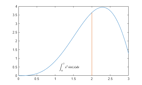

Create Plot Titles, Tick Labels, and Legends with LaTeX

MATLAB allows you to use LaTeX markup to format plot titles, tick labels, and legends for more sophisticated mathematical expressions. For example, you can create a plot displaying both a sine wave and a cosine wave with LaTeX formatting to enhance the readability and appearance of your graph.

Here’s an example:

x = -10:0.1:10;
y = [sin(x); cos(x)];
plot(x,y)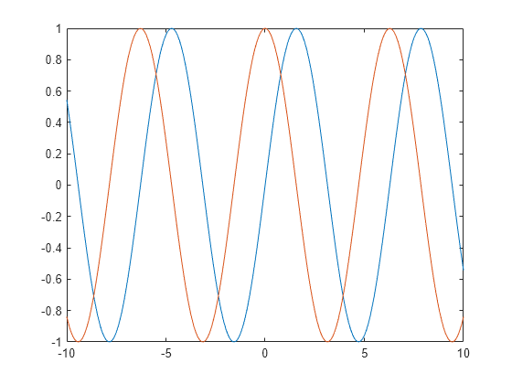

To set the x-axis tick values to multiples of pi, use the xticks function. Next, retrieve the current axes with the gca function, and set the TickLabelInterpreter property to ‘latex’ for LaTeX-style formatting. For inline expressions, enclose the LaTeX markup in single dollar signs ($).

xticks([-3*pi -2*pi -pi 0 pi 2*pi 3*pi])
ax = gca;
ax.TickLabelInterpreter = 'latex';
xticklabels({'$-3\pi$','$-2\pi$','$-\pi$','0', '$\pi$','$2\pi$','$3\pi$'});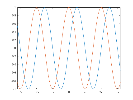

To add a title that includes LaTeX markup, use the title function and set the Interpreter property to ‘latex’. Similarly, you can create a legend with labels containing LaTeX markup.

% Add title
str = 'Estimates $\hat{\psi_1}$ and $\hat{\psi_2}$';
title(str,'Interpreter','latex')

% Add legend
label1 = '$\hat{\psi_1}$';
label2 = '$\hat{\psi_2}$';
legend(label1,label2,'Interpreter','latex')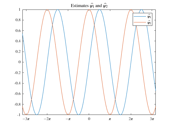

Conclusion

Incorporating Greek letters and special characters into your MATLAB chart text enhances readability and gives your plots a more professional appearance. By using LaTeX-style formatting or built-in MATLAB commands like \pi, \alpha, and \beta, you can display mathematical symbols and letters seamlessly within titles, axis labels, and legends. This ability to represent mathematical expressions and scientific notations directly in your plots ensures clarity and precision in communicating your data to others. So, whether you’re working with equations, variables, or scientific terms, mastering this technique will elevate your MATLAB visualizations.